Introduction
In real-world datasets, not all variable is numeric. Many are categorical — for example:
city: {Delhi, Mumbai, Chennai}education: {Graduate, Postgraduate, PhD}gender: {Male, Female}
But mathematical calculation can be done in numerics only, thats why machine learning models require numbers as inputs. That’s where categorical encoding comes in.
In this blog, we’ll explore the three most common encoding techniques :
One-Hot Encoding
Label Encoding
Target Encoding
and see how they behave in a regression task .
Dataset
Let’s simulate a simple dataset of house prices with a few categorical features.
Code
import pandas as pdimport numpy as npfrom sklearn.preprocessing import OneHotEncoder, LabelEncoderfrom sklearn.linear_model import LinearRegressionfrom sklearn.model_selection import train_test_splitfrom sklearn.metrics import r2_score, mean_squared_errorimport matplotlib.pyplot as pltimport warnings; warnings.filterwarnings("ignore" )
Code
# Create synthetic dataset 42 )= 1000 = pd.DataFrame({'city' : np.random.choice(['Delhi' , 'Mumbai' , 'Chennai' , 'Kolkata' ], sample_size),'furnishing' : np.random.choice(['Furnished' , 'Semi' , 'Unfurnished' ], sample_size),'size_sqft' : np.random.randint(500 , 2000 , sample_size),'price_lakhs' : np.random.randint(30 , 120 , sample_size)
0
Chennai
Semi
1295
93
1
Kolkata
Unfurnished
1472
39
2
Delhi
Furnished
1092
67
3
Chennai
Furnished
1637
110
4
Chennai
Furnished
1563
37
...
...
...
...
...
995
Delhi
Semi
1784
76
996
Delhi
Semi
1272
64
997
Kolkata
Semi
849
48
998
Kolkata
Furnished
1875
37
999
Chennai
Furnished
1019
55
1000 rows × 4 columns
0️⃣↔︎️1️⃣ 1. One-Hot Encoding
One-Hot Encoding creates a new column for each category. Each row gets a binary (0 or 1) depending on whether the category applies.
Code
# one-hot encode = data.copy()= OneHotEncoder(sparse_output= False )= encoder.fit_transform(df_ohe[['city' ]])= pd.DataFrame(encodedObj, columns= encoder.get_feature_names_out(['city' ]))print (df_encoded.head())# combine with original dataframe = pd.concat([df_ohe, df_encoded], axis= 1 ).reset_index(drop= True )print (df_ohe.head())
   city_Chennai  city_Delhi  city_Kolkata  city_Mumbai
0           1.0         0.0           0.0          0.0
1           0.0         0.0           1.0          0.0
2           0.0         1.0           0.0          0.0
3           1.0         0.0           0.0          0.0
4           1.0         0.0           0.0          0.0
      city   furnishing  size_sqft  price_lakhs  city_Chennai  city_Delhi  \
0  Chennai         Semi       1295           93           1.0         0.0
1  Kolkata  Unfurnished       1472           39           0.0         0.0
2    Delhi    Furnished       1092           67           0.0         1.0
3  Chennai    Furnished       1637          110           1.0         0.0
4  Chennai    Furnished       1563           37           1.0         0.0

   city_Kolkata  city_Mumbai
0           0.0          0.0
1           1.0          0.0
2           0.0          0.0
3           0.0          0.0
4           0.0          0.0
Works best when the number of unique categories is small.
Avoid if the column has many unique values — it leads to the curse of dimensionality.
🔠↔︎️🔢 2. Label Encoding
Label Encoding simply assigns a numeric label to each category.
Code
# label encode = data.copy()= LabelEncoder()= encoder.fit_transform(df_le[['city' ]])# get mapper print (dict (zip (encoder.classes_, encoder.transform(encoder.classes_))))= pd.DataFrame(encodedObj, columns= ['city_le' ])print (df_encoded.head())# combine with original dataframe = pd.concat([df_le, df_encoded], axis= 1 ).reset_index(drop= True )print (df_le.head())
{'Chennai': np.int64(0), 'Delhi': np.int64(1), 'Kolkata': np.int64(2), 'Mumbai': np.int64(3)}
   city_le
0        0
1        2
2        1
3        0
4        0
      city   furnishing  size_sqft  price_lakhs  city_le
0  Chennai         Semi       1295           93        0
1  Kolkata  Unfurnished       1472           39        2
2    Delhi    Furnished       1092           67        1
3  Chennai    Furnished       1637          110        0
4  Chennai    Furnished       1563           37        0
Models may interpret the numeric labels as ordinal (i.e., ordered), even when they’re not. That can mislead linear models like regression.
Works fine for tree-based models (e.g., RandomForest, XGBoost).
Avoid for linear regression, SVM, or distance-based models.
🎯↔︎️🔢 3. Target Encoding
Target Encoding replaces each category with the average value of the target variable (like price).
Code
= data.copy()'city_target' ] = df_te.groupby('city' )['price_lakhs' ].transform('mean' )'city' , 'price_lakhs' , 'city_target' ]]
0
Chennai
93
74.900862
1
Kolkata
39
75.878571
2
Delhi
67
70.445736
3
Chennai
110
74.900862
4
Chennai
37
74.900862
...
...
...
...
995
Delhi
76
70.445736
996
Delhi
64
70.445736
997
Kolkata
48
75.878571
998
Kolkata
37
75.878571
999
Chennai
55
74.900862
1000 rows × 3 columns
Great for high-cardinality features (many unique categories).
Risk of data leakage — use it only within cross-validation folds.
⚖️ Comparing Impact in a Regression Task
Let’s see how encoding affects a simple linear regression model.
One-Hot Encoding
Code
# Use one-hot encoded data for regression = df_ohe.drop(columns= ['city' ,'furnishing' ,'price_lakhs' ])print (f"Independent variable/Feature(s): { list (X.columns)} " )= df_ohe['price_lakhs' ]print (f"Dependent variable/Target: { y. name} " )= train_test_split(X, y, test_size= 0.3 , random_state= 42 )# training = LinearRegression()# prediction = model_ohe.predict(X_test)print (pd.DataFrame({'Actual' : y_test, 'Predicted' : np.round (preds_ohe, 2 )}).head())# evaluation = r2_score(y_test, preds_ohe)= mean_squared_error(y_test, preds_ohe)print (f"""R² Score: { r2_ohe:0.6f} , MSE: { mse_ohe:0.6f} """ )
Independent variable/Feature(s): ['size_sqft', 'city_Chennai', 'city_Delhi', 'city_Kolkata', 'city_Mumbai']
Dependent variable/Target: price_lakhs
Actual Predicted
521 108 75.04
737 48 70.66
740 113 75.08
660 112 76.98
411 69 77.28
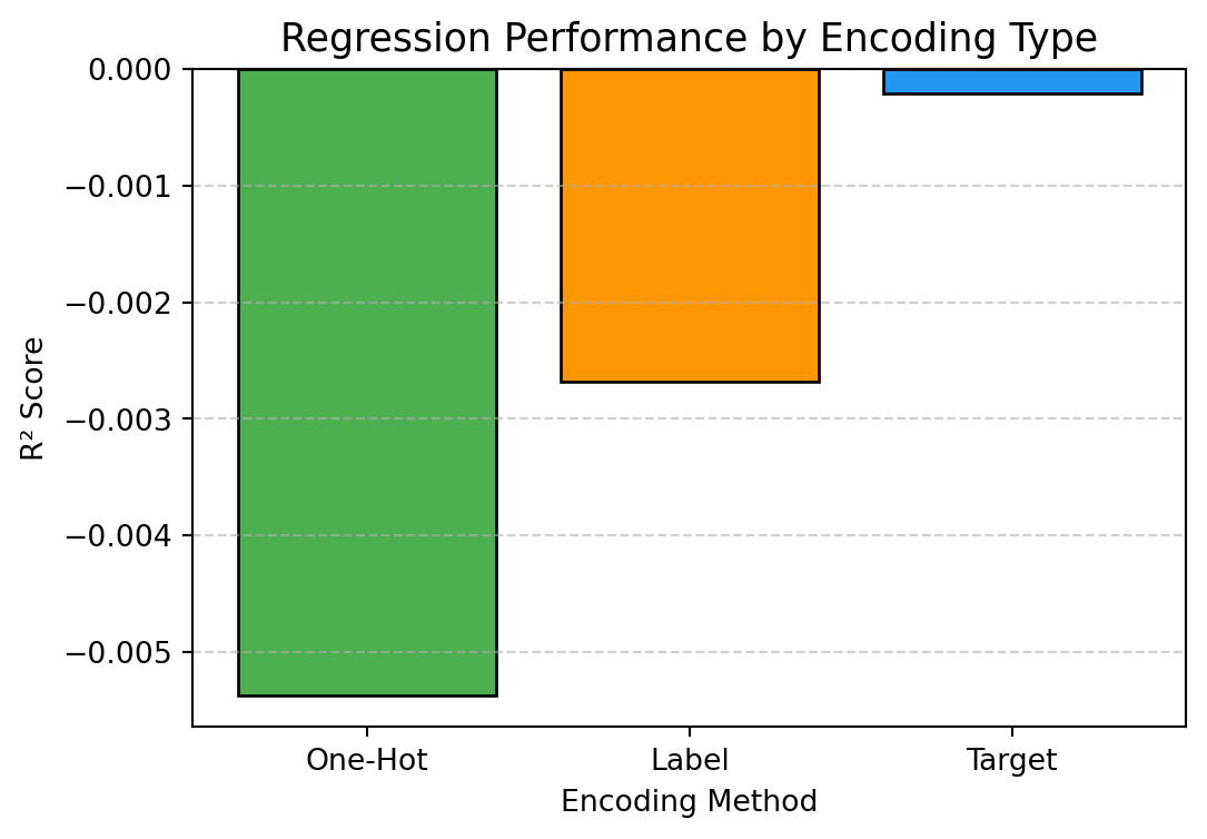
R² Score: -0.005375, MSE: 673.276323
Label Enconding
Code
= df_le.drop(columns= ['city' ,'furnishing' ,'price_lakhs' ])print (f"Independent variable/Feature(s): { list (X.columns)} " )= df_le['price_lakhs' ]print (f"Dependent variable/Target: { y. name} " )= train_test_split(X, y, test_size= 0.3 , random_state= 42 )# training = LinearRegression()# prediction = model_le.predict(X_test)print (pd.DataFrame({'Actual' : y_test, 'Predicted' : np.round (preds_le, 2 )}).head())# evaluation = r2_score(y_test, preds_le)= mean_squared_error(y_test, preds_le)print (f"""R² Score: { r2_le:0.6f} , MSE: { mse_le:0.6f} """ )
Independent variable/Feature(s): ['size_sqft', 'city_le']
Dependent variable/Target: price_lakhs
     Actual  Predicted
521     108      74.01
737      48      74.04
740     113      74.03
660     112      74.00
411      69      74.18
R² Score: -0.002678, MSE: 671.469921
Target Enconding
Code
= df_te[['city_target' , 'size_sqft' ]]print (f"Independent variable/Feature(s): { list (X.columns)} " )= df_te['price_lakhs' ]print (f"Dependent variable/Target: { y. name} " )= train_test_split(X, y, test_size= 0.3 , random_state= 42 )# training = LinearRegression()# prediction = model_te.predict(X_test)print (pd.DataFrame({'Actual' : y_test, 'Predicted' : np.round (preds_te, 2 )}).head())# evaluation = r2_score(y_test, preds_te)= mean_squared_error(y_test, preds_te)print (f"""R² Score: { r2_te:0.6f} , MSE: { mse_te:0.6f} """ )
Independent variable/Feature(s): ['city_target', 'size_sqft']
Dependent variable/Target: price_lakhs
     Actual  Predicted
521     108      75.00
737      48      70.18
740     113      75.04
660     112      76.31
411      69      76.63
R² Score: -0.000205, MSE: 669.813730
Comparison
Code
# Compare R² across encoders = pd.DataFrame({'Encoding' : ['One-Hot' , 'Label' , 'Target' ],'R2_Score' : [r2_ohe, r2_le, r2_te],'MSE' : [mse_ohe, mse_le, mse_te]= (6 ,4 ))'Encoding' ], results_df['R2_Score' ],= ['#4CAF50' , '#FF9800' , '#2196F3' ], edgecolor= 'black' )'Regression Performance by Encoding Type' , fontsize= 13 )'Encoding Method' )'R² Score' )= 'y' , linestyle= '--' , alpha= 0.6 )
Code
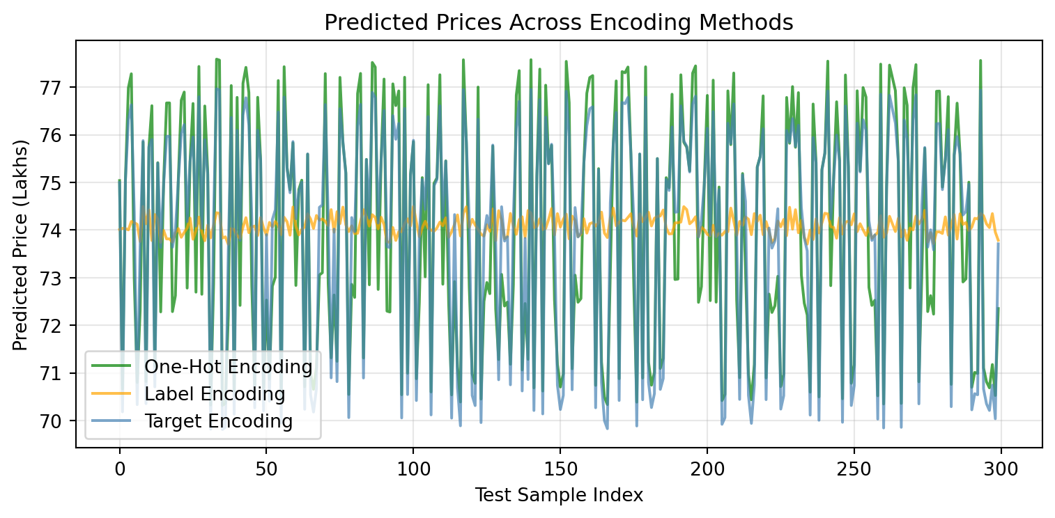
= (8 , 4 ))= 'One-Hot Encoding' , color= 'green' , alpha= 0.7 )= 'Label Encoding' , color= 'orange' , alpha= 0.7 )= 'Target Encoding' , color= 'steelblue' , alpha= 0.7 )"Predicted Prices Across Encoding Methods" )"Test Sample Index" )"Predicted Price (Lakhs)" )True , alpha= 0.3 )
It shows predicted prices (in lakhs) for test samples indexed from 0 to 300 on the x-axis. The y-axis ranges roughly from 70 to 78 lakhs.
Three different encoding methods are compared:
One-Hot Encoding (green line) with high fluctuation in values between about 70 and 77 lakhs.
Label Encoding (orange line) which is very stable around 74 lakhs.
Target Encoding (blue line) which fluctuates between about 70 and 77 lakhs, somewhat similar to one-hot encoding but with different patterns.
The plot clearly demonstrates how predicted price variance differs depending on the encoding method used for the test samples. Label encoding leads to the most stable price predictions, while one-hot and target encoding lead to more volatile predictions.
🧭 Summary
One-Hot Simple, interpretable
High dimensionality
Small categorical sets
Label Compact, easy
May imply order
Tree-based models
Target Handles many categories
Risk of leakage
Large datasets, regularized models
Categorical encoding isn’t just preprocessing — it’s part of feature engineering intelligence. A good choice of encoding can make or break model performance.
Next time you face a categorical column, remember: “Encoding is not just transformation — it’s translation.”